I would like to show the results of a major breakthrough in the study of crime. Recall that the age crime curve was discovered by Quetelet in 1831. Since then, many people have tried to understand why it occurs. These attempts have resulted in failure because the age crime curve is a “cluster problem.” That is, there are multiple major conceptual issues that need to be addressed to solve the age crime puzzle. I was able to find the solution to one piece of the puzzle, which I will discuss here, and this permits one to find the solution to the rest of the age crime puzzle.
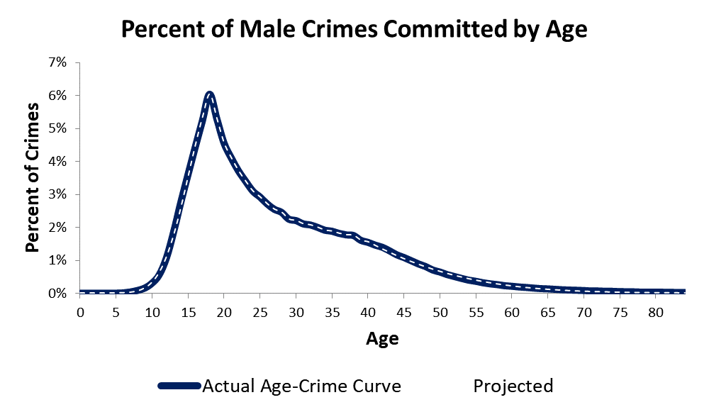
The plot shown above has the results from my age crime curve calculations. The blue line is the actual age crime curve. The estimates I found for the age crime curve are represented by a white dashed line. Note that the age crime curve estimates are almost exactly the same as the actual age crime curve. The accuracy of my model exceeds an R Squared of .9995. I will go into the reasons why below.
I am not bragging when I call these findings a major breakthrough. The age crime curve is like a Rosetta stone for criminology. In 1983, Hirschi and Gottfredson, two of criminology’s top scholars, noted that “When attention shifts to the meaning or implications of the relation between age and crime, that relation easily qualifies as the most difficult fact in the field.” If we can’t explain the age crime curve, we are missing a major piece of the causal puzzle of crime.
The Age Crime Curve is a Cumulative Distribution Function
My theory about the cause of the age crime curve was that the age crime curve was a developmental artifact. This was also Quetelet’s theory in 1831. He suggested that this conclusion was obvious.
I developed this conclusion separately while studying life course development. Research had shown that crime is inversely related to intelligence. Research had also shown that muscular people commit more crimes that non-muscular people. Might these two facts help explain crime by age? We know that strength and intelligence are both changing over the life course. What if the development of intelligence lags the development of strength?
This was my working hypothesis: The development of mental capacity over the life course lagged the development of strength over the life course, and the developmental lag between strength and mental capacity caused the age crime curve.
I will dive deeper into my lagged developmental theory in future weeks. There was a problem that I had to address first. The data made no sense.
The problem I had with the actual age crime curve data was that my theory predicted that the age crime curve in the period from age 0-18 should be a straight line plot. My theory also predicted that crime rates from 46-84 should be falling linearly. If my theory was correct, crime rates should be rising linearly from 0-18 and falling linearly from 46-84. If you look at the actual age crime data in the plot above, you will see that the plot sections from 0-18 and from 46-84 are rising and falling curved lines and not straight lines. Why?
I eventually realized that the problem with lack of straight line plots was related to the fact that the propensity for crime by age from 0-84 is a set of 84 normal probability distributions and the age crime curve was a set of 84 points from 84 cumulative distribution function points.
Recall that in Week 7, I demonstrated how probability density functions are related to cumulative distribution functions.
Week 7: Cumulative Distribution Functions
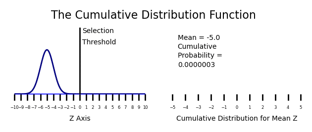
A cumulative distribution function is a sigmoid curve that results when a probability density function passes a threshold. The value of the cumulative distribution function is the area under the curve that is selected. See the animated version of the creation of cumulative distribution functions below.
In the case of the age crime curve, the threshold was the perceived difference between crime and non-crime. Note that, theoretically, crimes are severe harms. There are many types of harm that people commit. When the harm exceeds a certain level, the legal system generally categorizes that behavior as crime. In this case, the propensity for crime (harming others) is normally distributed and the criminal justice system selects the act that they call “crimes”, creating a threshold.
If you look at the male age crime curve shown above, you see that the sections of the age crime curve from 0-18 and from 46-84 are sigmoid shaped plots. My question was, are these sections sigmoid curves representing a cumulative distribution function? Was there a propensity/selection process?
To avoid confusion, please note that the section of the age crime curve from 19-45 also seems to be a sigmoid shape, but the section from 19-45 is not sigmoid, it is an exponential decay curve. I will discuss the reasons for this exponential decay in future weeks. I want to focus this week on the age crime curve from ages 0-18 and 46-84.
The Age Crime Curve Math
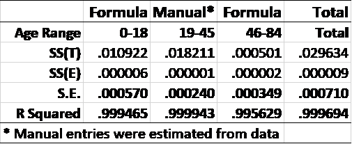
To test my theory that the propensity for crime rose linearly from 0-18 and dropped linearly from 46-84, I set up an Excel spreadsheet with the age crime rates by year. I split the age crime curve into three sections, 1) 0-18, 2)19-45, and 3) 46-84. Sections 0-18 and 46-84 were estimated using linear formulas and section 19-45 was estimated by minimizing the error by year.
I started out trying to find the linear solution for Z. Recall that a straight line formula for Z is Z = A + BX. In my case, A was the Intercept, B was the Slope, and X was Age.
I played with the slopes and intercepts for the Z score formulas from 0-18 and 40-84 until I found the best fits. The linear Z score formulas that fit best were as follows.
- 0-18: Z by Age = -5 + .3316*Age
- 46-84: Z by Age = -.79 – .0548*Age
I then calculated the crime rate for each Z score using Excel.
I found that the best fit required a constant in the formula. This was not unexpected since I was using percentage of crime by age, rather that actual crime rates. The constant was 13.778 and the estimated crime rate formula became.
Estimated Crime Rate by Age = p(Z by Age) / Constant = p(Z by Age) / 13.778
The results of these calculations are shown below. Note again that ages 19-45 were calculated manually and were not part of the model. The model generates an R Squared of .999465 from 0-18 and .995629 from 46-84.
The Probability of Crime by Age
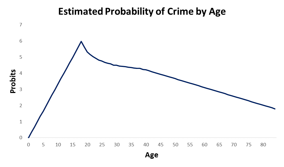
The results from the calculations described above appear to demonstrate convincingly that crime is normally distributed and that the age crime curve is a cumulative distribution function. If we transform the Z scores to Probits so that we can see the shape of the probability plot of crime by age, we get the following.
Note that the plot below is shown in Probits. The Method of Probits is a Z score transformation that was developed by Bliss in 1934. A Probit is a “probability unit” that is calculated by adding 5 to the Z score. The formula for a Probit is as follows.
Probit = Z + 5
The Probit transformation transforms the mean of a standard normal distribution from a mean = 0 to a mean = 5. The purpose is to avoid negative Z scores, which range from -5 to 5 for the standard normal distribution.
As an amusing aside, the Method of Probits was developed to make it easier to determine germ kill rates in the presence of antiseptics. This begs the question. What do germs and criminals have in common?
If my mathematical model for the age crime curve is correct, the probability of crime rises linearly from 0-18, drops in a curvilinear fashion from 19-45, and then drops linearly from 46-84. See below.
Conclusion
I hope the description of my discovery about the mathematical nature of the age crime curve makes some sort of sense. The age crime curve is a cumulative distribution function that is created by 84 individual normal distributions. One normal propensity distribution for each year of age.
Note that some people might question the high R Squared values I got. I have gone over this and it should not be a problem. I am using age crime data aggregated over millions of people over 10 years. This is population level data and is missing the variation present in individual data. This model shows the mathematical form of the age crime curve at the population level.
The point of my thesis is that logically, the age crime curve from 0-84 is a cumulative distribution function with 84 data points representing the crime rate for each age. If crime at each age is normally distributed, the crime rate at each age should be a point on a normal cumulative distribution function. That appears to be what I found.
These findings are logically consistent and they support a developmental theory of the age crime curve. More to come about that.
Note that this same model works as well for the female age crime curve. This model also fits the cumulative number of chronic conditions in a health propensity model.
These finding provide a statistical Rosetta stone in the sense that these data tell us that criminal propensity and health are normally distributed.
Questions?
Recent Comments