This week, I would like to introduce the issues related to cumulative distribution functions. There seems to be an almost universal lack of attention in the scientific literature given to the topic of cumulative distribution functions. Understanding cumulative distribution functions is essential to understanding the world around us.
The material for this week builds upon the material presented in the past two weeks of data pattern analysis, so if you have not read those posts, you probably should look them over. In particular, you should look at the Week 5 post on the healthcare dilemma. The Week 5 post provides a visual guide for the processes involved in creating cumulative distribution functions. These are variation and selection.
52 Weeks of Data Pattern Analysis: Week 5: The Healthcare Dilemma
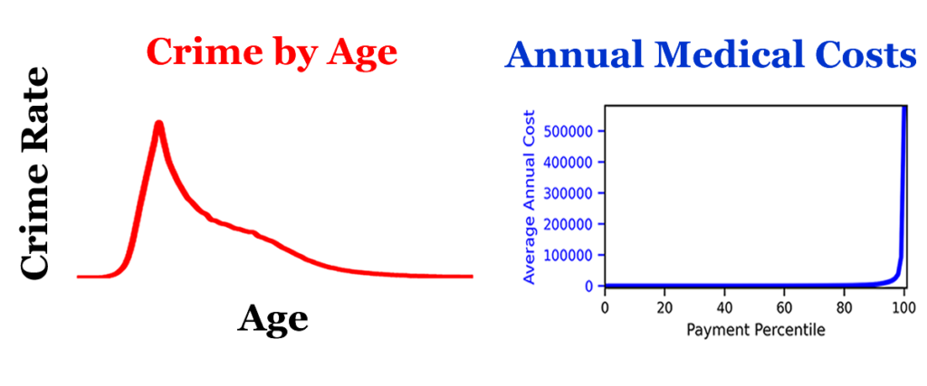
The lack of understanding related to cumulative distribution functions is a problem because we can’t solve the conceptual problems related to the age crime curve or the health cost curve without understanding cumulative distributions. Most of the data we consume consists of points on a cumulative distribution function, yet few people actually consider the properties of cumulative distributions.
A Quick Primer on the Math
Cumulative distributions are built by calculating sums of occurrences. In terms of the Calculus involved, the formula for a cumulative distribution function is an Integral. While it is not absolutely imperative that one understands the math, a quick primer may help the reader who is not familiar with this topic.
The Wikipedia article on Cumulative Distribution Functions is recommended.
Two Types of Cumulative Distributions
There are two types of cumulative distributions. Issues related to “the process of selection” distinguish the two types of cumulative distribution functions. The issues related to the process of selection seems to be almost universally ignored when discussing cumulative distributions.
In particular, we need to be aware of whether there is selection with replacement or selection without replacement.
- Cumulative distributions using selection without replacement
- Cumulative distributions using selection with replacement
I have not seen anyone write about cumulative distributions using selection with replacement, so I will save that for a future week. When working with cumulative distributions using selection without replacement, the cumulative distribution for the normal probability distribution is a sigmoid curve.
The outcome variable for cumulative distribution functions in selection without replacement is the sum of a binary variable with a 1 (selected) or 0 (not selected.) I understand that some would use logistic regression here. The outcomes are similar, but the theoretical explanations differ.
Thinking in Areas Under the Curve
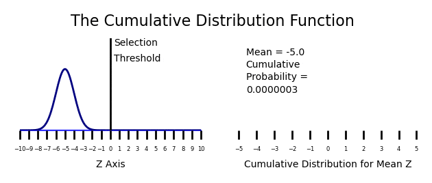
In both types of cumulative distribution function, the outcome is expressed as a rate. The cumulative rate can be modeled as the area under a curve. In the case of selection without replacement, the cumulative distribution can be modeled as the area under the normal distribution curve. This process is shown in the animated GIF shown above. The outcome for normal distributions is a sigmoid curve.
The sigmoid curve is only studied in a few disciplines. The disciplines where people use cumulative distributions from the normal distribution that come to top of mind are the following. If you want to add some, that would be welcome.
- Germ kill rates in the presence of antiseptics
- Diffusion of innovations
- Item response theory
I am going to argue that almost all disciplines that study living systems should use cumulative distributions to model processes. The problem that seems to be ignored with cumulative distributions is nonlinearity in outcomes with small selection rates. If one follows the animation over several iterations, you will notice that the rate of accumulation is greatest in the middle of the normal curve. There can be a change in the mean of several Z scores with very little change in the selection volume. This causes real problems when comparing rates of participation.
To illustrate the problems when comparing rates of participation, it will help to look at an example.
Male and Female Data Scientists
The problem with rate comparisons using cumulative distributions is that we need to think in terms of areas. The sum of the probabilities is the area under the probability distribution that is selected. See the animated GIF at the top of the page.
There is a highly nonlinear relationship between changes in the rate expressed as a percentage and changes in in the probability expressed as a mean change in the Z score. This is especially true when rates are small. To illustrate this, lets look at the differences in rates of male and female data scientists.
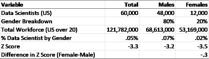
Approximately 80% of the data scientists are estimated to be male. This is about a 400% difference in the percentages expressed as a ratio. See the sample article below.
Why the World Needs More Women Data Scientists
If we calculate the differences in percentages in data scientist occupations between males and females at the population level, using the total US work force over 20 years old in the denominator, we see that the data scientist participation rates for males and females are both very low. Seven hundredths of a percent of the male US workforce (7 in 10,000 workers) are data scientists and 2 hundredths of a percent of the female US workforce (2 in 10,000 workers) are data scientists.
Comparing the Probability Density Functions
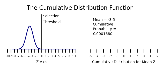
If we look at the differences between the probability density functions for males and females, we find that the differences are small. There is only a three tenths difference in the Z scores for the male and female populations in terms of the cumulative probability of becoming a data scientist.
Note that you can verify this for yourself using the NORV.S.INV function in Excel. Any inverse normal transformation function will work.
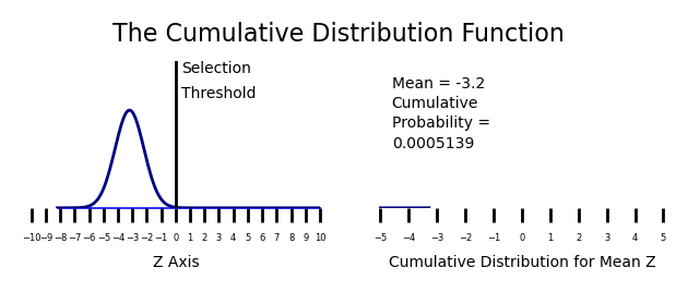
The mean female probability of becoming a data scientists is at -3.5 standard deviations and the mean male probability of becoming a data scientists is at -3.2 standard deviations.
Female Probability of Becoming a Data Scientist
Male Probability of Becoming a Data Scientist
The Unobserved Phenomena
Can you see the problem?
When people look at things like gender differences in the rates of employment for data scientists, they usually just look at the data they have on participation as a data scientist. They don’t look at the data on non-participation. The vast majority of the population (99.5%) has chosen to not become a data scientist. Probabilistically, the population differences in the probabilities of becoming a data scientist between the populations of males and females are very low.
Ignoring the cumulative distribution function in the population data occurs almost all of the time in almost every dataset that is presented. For example, I had to dig down into the US Bureau of Labor Statistics data to get actual real numbers of data scientists and even then, I had to estimate the percentages of males and females. If you search Google for gender differences in data science employment, it is almost impossible to find numbers. Almost all you can find are percentages.
Note that the scale shown above ranges from -10 to 10 standard deviations. This is because for a normal distribution with almost no participation, the normal probability distribution ranges from -10 to 0.
Think about this. Almost all of the data is unobserved.
Conclusion
This was intended to be an introduction to cumulative distribution functions. I hope that I have aroused some curiosity. How does this help explain the age crime curve or the health cost curve? How can we use this in “theory driven data science?”
It took me many years to wrap my head around this. Who thinks in areas? The only way that I was able to make sense of this was to visually explore the data.
Data Pattern Analysis.
Any input is welcome. Does this make sense? Can you see why this is important? What does not make sense?
Recent Comments